May 13, 2022

Last updated on Dec 1, 2020

A Primer on Probabilistic Methods in Engineering - Part 1

This primer gives a high-level introduction to probabilistic methods in engineering. This is of particular importance as we strive to improve our understanding of our engineering, and deliver increasingly optimised and efficient designs.

The bloomin’ weather

To start exploring probability let’s look at the weather, notoriously uncertain in the UK. Probabilities are a method to quantify uncertainty. The weather forecast reports the chance, or probability, of rain, say 20%, and this is something familiar to us.

A forecast with a 60% chance of rain expresses more certainty (of rain) than a forecast with a 20% chance of rain. This is obvious, yet a simple example of probabilities in daily life. Both forecasts use probabilities to express the uncertainty, and one forecast has (three times) more certainty of rain than the other.

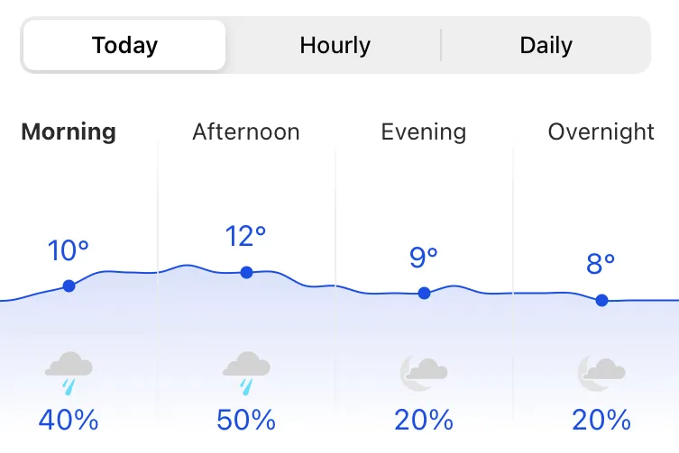
Weather forecasts are a good example of uncertainty in everyday life, and the use of probabilities

The middle ground

Something with a probability of 1, or 100%, is something with absolute certainty, it will happen. Similarly something with a probability of 0, or 0%, is something that will never happen, it’s an impossibility. Of course in reality most things are in the grey middle, not least the weather.

The probability spectrum is shown in the sketch below, from impossible (pigs might fly), to certain (we all will die). In the middle, as well as the weather in England, we also have a coin flip for an unbiased coin - something with a 50:50, or 50%, probability.

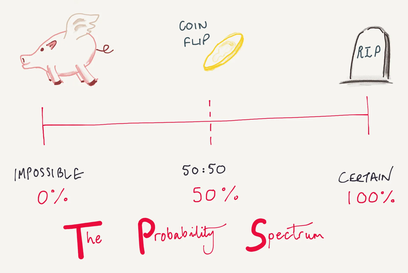
The probability spectrum (pigs might fly to death)

The conservative brigade

One approach to deal with uncertainty is of course to take the most conservative, pessimistic path. You can’t argue that this is conservative, but in doing so you lose all sense of just how ****conservative. Over-engineered is over-engineered… but how much, we are unable to quantify using this approach. Excess conservative is an issue that slowly undermines our understanding though, and propagates into all areas of a design. It can be hard to argue with the conservative brigade, because being overly conservative does result in a safe design, but just because it’s easy, it doesn’t mean it’s the best way, as we’ll see in more detail later.

The philosopher’s stone

Understanding probabilities and how to quantify uncertainty significantly improves our understanding of engineering performance. Probability is a tool, and like the philosopher’s stones, we use it to turn our base mental of conservative understanding into precious gold of enlightened wisdom in how our engineering works and performs. Ok, maybe it’s not quite as magical as that, but it’s still pretty useful.

The application of probabilistic techniques indicates what range of outcomes could occur, and with what chance, rather than blindly designing against an incredibly remote combination of loads (like the conservative brigade), with no understanding of the risk, in the belief that the resulting design must then be safe.

Besides the somewhat tenuous philosopher’s stone properties, why else would you use probabilistic methods? I’m glad you asked. It boils down to three points:

Improves understanding: Margins quantified on a reliability basis (understand uncertainty and understand true margin for a given reliability)
Enables trading: Trading of margin unlocked (i.e. where to target improvements / relaxations)
Improves value: Efficient use of data (measurement, construction, inspection, and resources directed to where they are most effective)

To take these in turn:

Improves understanding:
- Understand the most likely performance and bounds of performance
- Be able to respond to design challenge and changes by understanding the behaviour
- Understand the margins to failure
- The statistical or probabilistic treatment is directly related to the reliability
- Reduces sensitivity to variation in input parameters - a percentile output quantity is much less sensitive an output than a deterministic and conservative upper bound
- Improved understanding informs the placement of sensors, specific measurements, targeted inspections - the worth of data gathering is known
Enables trading:
- Engineering solutions that can be demonstrated as ALARP (As Low As Reasonably Practicable) - the realistic safety benefit can be understood in comparison to the time, cost and trouble of implementing
- Trading of margin unlocked so that targeted improvements or relaxations can be made
- Can optimise the design on a reliability basis
Improves value:
- Efficient and optimal engineering designs
- Avoids over-design
- Value for money where limited resources are targeted to where they are most effective

We use our philosopher’s stone to realise these benefits by making estimations, forecasts, and predictions of what is unknown (but knowable). Often this is based on an idealised understanding, but nonetheless we can use this to make useful predictions and improve our understanding.

Absence of evidence is not evidence of absence, and as engineers the burden of proof is on us to show that we understand the behaviour and performance of what we’re designing.

On uncertainty

Uncertainty is doubt. It could be caused by measurement uncertainty, random events, lack of knowledge, and others.

Uncertainty can be categorised in the following ways, (with the first two being the two below of most practical importance):

Epistemic
- Lack of knowledge uncertainty
Aleatory
- Inherent randomness uncertainty
Semantic
- Linguistic uncertainty
Ontological
- Belief system uncertainty

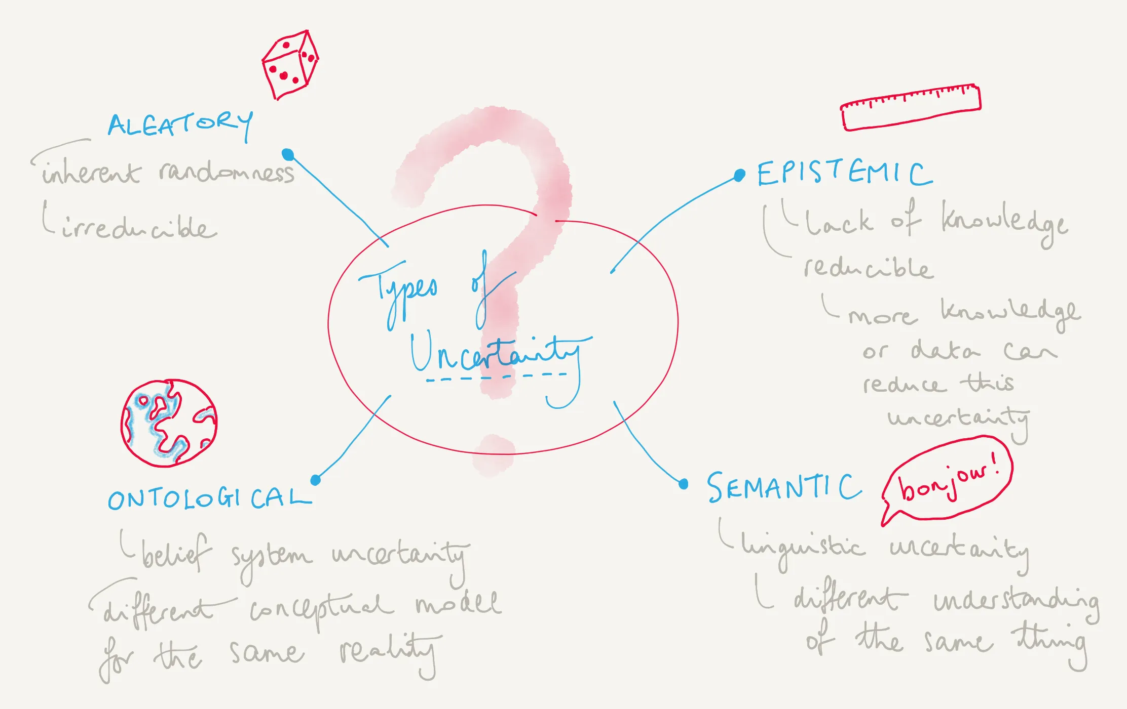
Types of uncertainty

The two significant types of uncertainty are explored a bit further below, since this will be crucial to our understanding of our engineering. And later we’ll see how to quantify uncertainty, and make predictions.

Epistemic uncertainty

Epistemic **uncertainty reflects our lack of knowledge. I could estimate your height is between 1m and 2m, and this range defines my uncertainty. I could improve matters by adding knowledge, for example measuring your height with a tape measure. Even then, there is still some uncertainty, but instead of being +/-0.5m it’s now +/-0.5cm. Much better. The important thing here is that with epistemic uncertainty we are able to reduce the uncertainty with more knowledge, data or information.

As well as measurement uncertainty this would also encompass ranges of values for parameters, a range of viable models, the level of model detail, multiple expert interpretations, and statistical confidence.

Aleatory uncertainty

Aleatory uncertainty represents inherent randomness. A coin toss is inherently random, an example of aleatory uncertainty, and this type of uncertainty is irreducible- it cannot be reduced by the accumulation of more data or additional information.

Since aleatory uncertainty cannot be reduced it must be tackled by having sufficient margin. Think of margin as how far away you are from the brink!

Crazy pendulums

We’ve seen the types of uncertainty, now let’s work through some example of how can quantify that uncertainty.

All systems must behave according to the laws of physics, but that doesn’t mean we can perfectly predict them. We’ve already talked about the weather, but I’ll also illustrate this point using an example closer to engineering; the double pendulum. We know the equations of motion for a double pendulum system and if we know precisely the initial conditions then we can perfectly predict the resulting behaviour. The issue however here is in measurement uncertainty (epistemic). A double pendulum system is so sensitive to the initial conditions that a very small measurement error results in vastly different responses. The response is highly asymmetric (a topic for another day).

The purpose of the double pendulum example is also to show that uncertainties can be quantified numerically. And, by extension, it shows that we can reduce response uncertainty by reducing measurement uncertainty. This is an epistemic uncertainty which as we’ve seen is a reducible uncertainty, reducible with more knowledge.

The animation below shows 100 double pendulums with ever-so-slightly different initial conditions. This soon manifests itself in a considerably different response. And by slightly different initial conditions I mean that I have sampled the initial angle for the 100 double pendulums from a normal distribution (more on that later) with a mean of 135 degrees and standard deviation of just one thousandth ****of a degree.

100 double pendulums with very slightly different initial angles

In summary, a tiny variation (or uncertainty) can have significant implications.

The double pendulum example above is something that I have created in a Jupyter Notebook, an interactive notebook environment, and this is something that you can explore too.

The animation above may be fun to watch, but say we were interested in an output of this system, the angular velocity say. And we have an inkling that the system is sensitive, so we want to use an upper bound angular velocity with a probability of 95%. Our weather equivalent of a pretty certain rainy day.

In this pendulum example there are input parameters or variables. Parameters like the initial angle, the mass of the pendulum bobs, and the lengths of the pendulum arms. These parameters might be measured, and that of course would be subject to some measurement error. And measurement error tends to follow a normal distribution…

The New Normal

To explore the normal distribution, think about a commute. In COVID-19 times this may be considerably shorter, but a commute can be approximated as a normal distribution, that is, you have an average commute (say 30 minutes), but there is some uncertainty, and actually it varies either side of this. If we were to draw a graph with the x-axis representing the commute time, then the y-axis representing the probability or likelihood of that commute time occurring on any given day. It would look like a bell-shaped curve. The most likely commute is the mean value - the peak of the bell curve. But sometimes there are “tail events”, referring to the tails of the bell curve, which are unlikely but where the commute time might be horribly long due to a pileup on the A38, or unusually short getting to the office during lockdown. The figure below shows this, and a normal distribution is described by just two numbers - the mean (the peak) and the standard deviation (a measure of the spread).

A normal distribution - a bell-shaped curve, also called a Gaussian distribution.

Randomly picking from a normal distribution there is a 95% that you’ll be within 1.96 standard deviations of the mean. So for your commute with a mean of 30 minutes, if this had a standard deviation of 5 minutes then 95% of your commutes to work would be between about 20m:12s and 29m:48s. In this example there is a ~1 in 1000 chance that the commute is 45 minutes or more.

Back to the example of the double pendulum, the uncertainty here is due to epistemic uncertainty, and we could expect to reduce the uncertainty by improving our knowledge, by measuring with improved accuracy.

With the double pendulum example, we can run the model with the exact input parameters:

Initial angles of 135 degrees
Initial velocities of zero
Both masses being 1 kg
Both lengths being 1 m

And we’ll get an answer, 17.45 rad/s as the maximum absolute angular velocity. Neat.

But our measurement of the input parameters is not perfect. We’ll just explore a single parameter, but this would equally apply to the uncertainty present in all the parameters. With the initial angles parameter the animation earlier showed that a tiny 1 in 1000th of a degree change made a crazy dance of it. If we run our simple double pendulum model hundreds of time, each time with a slightly different value of the initial angles we can understand the effect on the results, the angular velocity in this case.

So let’s do that. The initial angle is given as a normal distribution with a mean of 135 degrees and a standard deviation of 0.001 degrees. We can sample (the metaphorical close your eyes and put your hand in the sweetie jar) and pull out a value for the angle, say 135.00056, run the model, and get an angular velocity. We repeat this 1000 times, and then get a distribution of angular velocities, looking something like the graph below (although will of course be different each time due to the randomness of the sampling).

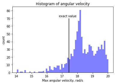
So we can see that a very slight change in initial angle gives a range of the maximum absolute angular velocity anywhere between 14 rad/s and 20 rad/s! Sensitive or what!

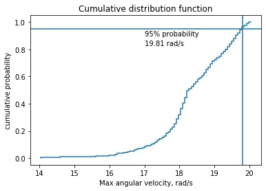
Instead of the histogram plot above, we can instead more helpfully plot this as a cumulative distribution function (CDF), which will show our angular velocity vs. the cumulative probability. This is shown below and means we can do useful things like read off the 95% probability. For this example, the angular velocity that bounds 95% of the expected cases is 19.81 rad/s.

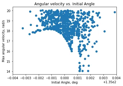
And to reflect back on the conservative brigade; in some cases it may be clear cut what parameter values will give a conservative design, but this pendulum example shows that this isn’t always the case. Even with this simulation model, it’s not easy to guess the conservative initial conditions. A plot of initial angle against the maximum angular velocity (see below) shows there is now correlation, no “conservative” initial angle to give a conservative response. The conservative brigade would in this case be marching right off a cliff.

Crazier weather

The double pendulum was an example of epistemic uncertainty, and sensitivity in general really. For an example of aleatory uncertainty we’ll turn back to the weather. Where rain drops land is something that is inherently random. That is, even with more knowledge (better measurements) we cannot reduce this inherent randomness, and during rain the chance of a rain drop hitting any given location, within say a pond or lake, is random, inherently random. If we divided our pond into say a 100 x 100 grid, given a rain drop the chance of it hitting any grid square is 1 in 10,000. And there’s nothing we can do about it, except where a coat.

The animation below does just this, showing the rain drops hitting randomly on the surface of our pond.

Inherently random raindrops

As well as the rain, there are other events which are inherently random that are more applicable to engineering, events like earthquakes, floods and extreme wind. Typically these are described by a return period - a recurrence interval - for example a 1 in 100 year flood, A 1 in 100 year flood is a random event, with a probability of occurring that is inherently random, it is an example of aleatory uncertainty.

Casino gambles

Back to a more general approach now. In the general case, quantifying uncertainty involves assigning probabilities, that is likelihoods to a parameter, model, property, event occurring. We’ve already seen examples of this with the normal distribution used to represent the measurement uncertainty in the pendulum example, or the rain drop random event probability.

And of course our general probabilistic methods mean we can account for and quantify the presence of both types of uncertainties (aleatory and epistemic) on our engineering.

Before we go into a framework for probabilistic methods, it’s worth just reminding ourselves that:

Essentially all models are wrong, but some are useful

Any model is built upon assumptions, conservatisms, non-conservatisms and uncertainties. We must always remember this, but the beauty is that probabilistic tools can help understand and quantify this in a systematic way.

We already saw how we ran the double pendulum model hundreds of times to get an distribution of the output. This method is more generally called the Monte Carlo method. Monte Carlo methods were first developed to solve problems in particle physics at around the time of the development of the first computers and the Manhattan project for developing the first atomic bomb. The name Monte Carlo refers to the casino and gambling being the random sampling that we did in the example earlier. It uses the law of large numbers which says that the more samples we take the more we converge on the expected value.

We sample the input parameters, run the model, which then propagates the uncertainty to the output parameters.

Here’s the general probabilistic framework:

Construct analytical model (e.g. finite element model, numerical model) ← this is something we would do as engineers anyway
Monte Carlo sampling of input distributions, run model, obtain output response
Compare with acceptance criteria ← this is something we cover in more detail later

If Step 1 above involves a computational expensive model, that is, one that takes a long time to run, then we can “fit” an estimator to the model, and then sample from the estimated model (sometimes called a surrogate model, a metamodel or a response surface). This means we can run the time-consuming model only a handful of times, but still sample thousands of times from the resulting surrogate model. Think of the surrogate model / response surface as a line-of-best-fit - it means we can estimate the output at any point. It gets a bit fun to imagine since actually the response surface is a surface-of-best-fit in N-dimensional space…

The framework then looks like this:

Construct analytical model (e.g. finite element model, numerical model)
Select set of design points and run model for this set (e.g. using a Design of Experiments approach)
Fit a surrogate model (also called a response surface) to design point runs
Monte Carlo sampling of input distributions against response surface to obtain output response
Compare with acceptance criteria

This extended framework is shown in the figure below.

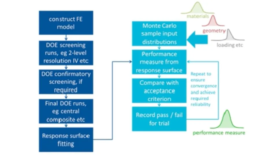
Probabilistic framework

How safe is safe enough?

The primary issue with all uncertainties is the communication of the risk created by the aleatory and epistemic elements. We take chances every day, in fact the probability of dying in a road accident in any given year is about 1 in 20000, or 0.005%. Over a lifetime, the probability is 1 in 240, or 0.4167%. Once we know the probability, or risk, we can make an informed decision about whether the risk is acceptable. This applies whether we’re deciding on whether to get in a car, or whether we’re deciding on if we need a brolly, or even if our engineering structure is safe enough.

In the pendulum example we used a probability of 95% to give our upper bound for the maximum angular velocity. This was somewhat arbitrary, but if we designed to this value there would be a 5% probability of failure, assuming no additional margins. The exact percentile confidence level will be selected to provide the necessary reliability for a given performance. When limited to a deterministic approach it is difficult to justify anything other than the most conservative combination of parameters, however the probabilistic approach allows the use of a design value appropriate to the required or agreed confidence level. This utilises similar ideas to all modern design codes which aim to achieve designs with a minimum level of reliability.

Book end

That’s a brief summary. We’ve covered:

Probability is a tool to quantify uncertainty
The framework for probabilistic methods is simple and applicable to any situation that can be modelled
Probabilistic methods propagate the input parameter uncertainties through to the output parameters giving an improved understanding of the performance
Uncertainty is everywhere, so if you can’t beat ‘em, join ‘em

To dig deeper, explore the interactive notebooks. And as for what’s next, I would like to go into more detail on surrogate modelling, since this is a topic in its own right.

Until then, bon chance.

Nick Stevens, November 2020

Resources

Jupyter Notebook

The Jupyter notebook below is an interactive notebook where you can run and explore the code yourself. You can run this locally, or can use something like Google Colab, both options are free.

Download Jupyter Notebook (Primer_probabilistic_methods_Part1.ipynb)